Correlation using Parasequences; parasequence sets; and systems tracts

As demonstrated by the exercises that follow, the interpretation of carbonates can be enhanced by first identifying the parasequences, or cycles (Pomar, 1991; and Pomar and Ward, 1994, 1995, 1999), in cores and well logs that penetrate the section being studied. Van Wagoner et al., (1990) were among the first to recognize that parasequences boundaries can be easily correlated regionally, and coincidently represent good time markers. Van Wagoner et al., (1990) also reasoned that carbonate parasequences were deposited when the rate of accumulation exceeded the rate at which accommodation space developed; they argued that a parasequence boundary (mfs) formed when the rate at which accommodation space was created exceeded the rate of sediment supply ("give-up") and there is termination of the carbonate factory. The difference in the character of each parasequences reflects: 1) differences in the behavior of the relative sea level during sediment deposition, particularly when there were abrupt changes of the sea level and: 2) the position of the geographic location of the depositional setting within the systems tract.

The figure to the left illustrates some typical parasequences found throughout the section used in the exercises with their predicted depositional settings and occurrences within the sequence (click figure to expand).

In left x-section (click figure to expand), the ideal parasequence is based on the observed lithofacies succession.

Correlation Based on Stacking patterns & Log Character

Each of the suites of well logs provided in the exercises includes gamma ray, porosity, permeability, sonic, density, and other log information. Additionally, the data set for each well includes a lithofacies analysis made from cored portions of the wells (see Exercise 1).

Having first identified the parasequences in the cores and well logs of the exercises the second step in your interpretation will be to analyze the stacking pattern of vertical recurring cycles of coarsening or fining upwards sediment. These patterns are used to identify the progradational, aggradational and retrogradational character of the section which in turn lead to the identification of lowstand system tracts (LST), transgressive system tracts (TST) and highstand system tracts (HST) that are enveloped by the mfs, TS and SB. As in clastics the parasequence cyclic stacking patterns in carbonates are commonly identified on the basis their variations in grain size.

The Bounding Surfaces that Bound and Subdivide Parasequences of the Wells in the Exercises

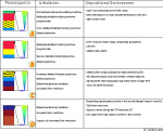
The surfaces listed below can be seen in the cores and well logs of the exercise materials. You should note that there are no type 1 sequence boundaries in these sections

How major surfaces are identified using lithofacies character

Shelf-margin wedge (SMW) sequence boundary, type-2 (SB-2)
If the SMW SB-2's of the exercise data set are examined and compared to the other system tracts they will be found to be relatively thin and so the adjacent sequence boundary may be ambiguous. For this reason the best means of identifying this boundary is by looking for marked changes in the trends shown by the stacking patterns. Goldhammer et al. (1991) noted that a SB-2 usually develops during a time at which there is a maximum decrease in the rate of development of long-term accommodation. This occurs when is a turn around occurs from progressively thinning upward cycles to thickening upward cycles. Thus a SB-2 is to be identified on the basis of the character of stacking patterns including cycle thickness, facies character, lateral geometry, and early diagenetic attributes (Goldhammer et al., 1991) (Figure)

Transgressive or Drowning Surface (ts)
This surface marks the sudden deepening (increase of relative sea level) and the termination or decrease in the deposition of shallow lithofacies while there is increase in the thickness of deeper water lithofacies. This surface is often marked by a hardground and or Glossifungites burrows and borings. Sometimes a reworked gravel of the shallow sediment lies on this surface.

The Maximum Flooding Surface (mfs)
The best means to identify the mfs within shallow part of the basin (outer ramp) is to identify a definite change in stacking pattern in which the cycles change from deep facies (wackestone and packstone dominated) into shallow facies (skeletal intraclasts). This geometrical trend can also be observed as it moves laterally shelfward.

How major surfaces are identified using well log character

Shelf-margin wedge (SMW) sequence boundary, type-2 (SB-2)
An SB-2 is identified by an abrupt Gamma Ray spike (high), which corresponds to an increase in porosity either within the shelf margin or the basin region

Transgressive or Drowning Surface (ts)
The drowning surface can also be identified by an abrupt gamma ray log spike (high) marking deepening (significant change in lithology); an increase of sonic velocity; and sudden decrease in porosity to very low values (5% or less) throughout the section. All these properties are indicators of a sudden deepening in the depositional setting (increase of relative sea level).

The Maximum Flooding Surface (mfs)
An mfs is identified in the section by an abrupt gamma ray spike of logs from wells within the basin. It should be noted that an mfs becomes increasingly difficult to identify within sediments were deposited close to and within the shelf setting since in these localities only contain shallow shelf carbonate facies and no radioactive shales are present. Despite this lack of shale a gamma ray spike can still be recognized, particularly where this has been amplified to aid in its identification.

Fischer Diagrams

Fischer plots can be used successfully to extract the 3rd-order and higher sea level fluctuations from high frequency cycles identified on the section. These plots illustrate long-term accommodation changes similar to those described by Goldhammer et al. (1991) and "reveal systematic changes in accommodation by plotting successive deviations in cycle thickness from the average cycle thickness" (Read and Goldhammer, 1988). Fischer diagrams (plots) can be constructed to build third order sea level curves that can then be comparing to the Haq et al (1987) sea curve. Another important use for these plots is to establish the role of subsidence within the depositional setting. This is achieved by comparing plots for different localities within a basin. The wells selected for the exercise penetrate the shallowest portion of the section. Selecting wells to make Fischer plots from the deep water parts of the basin does not work out so well. This is because though the lime mudstone parasequences that form the basin fill have a cyclic character it is difficult to establish their relationship to water depth or time, key components to the Fischer plot.

The Fischer plots should be constructed based on the assumption that each cycle (parasequence) was deposited over times of equal duration and their subsidence rate were linear (sedimentation = subsidence). Any deviation from the horizontal datum reflected either eustatic sea level change or changes in subsidence rate (Read and Goldhammer, 1988). Since the duration in which these carbonate were deposited was relatively short, it is logical to infer that the primary controlling factor that lead to these deposits was short-term eustatic sea level fluctuation. The average cycle period (time/number of cycles) can also be determined if an exact duration is determined for any part of the section. For shallow water carbonates that experience exposure the cycle thickness can be used to infer a rise in the relative sea level and an increase in the resultant accommodation space.

The sea level curve rise-fall that can be determined from the Fisher Plots can be used to illustrate the relationship between sea-level changes and cycle thickness in response to the creation of accommodation space. The two diagrams provided with the exercises clearly show that during a sea-level rise, the cycle thickens; on the other hand, when sea level falls, the cycle thins.

Fourth-order sequences can be identified from the constructing the Fischer diagrams. Each of these sequences is bounded by a type-2 sequence boundary and is recognized on the diagram at the maximum sea level fall inflection point. Each of the 4th order sequences has a recognizable maximum flooding surface.

The Exercises

Now click on the highlighted exercises link to access exercises in the analysis of parasequences using well logs and cores that use major surfaces that include TS (transgressive surface), mfs (Maximum Flooding Surface), and SB (sequence boundary). Then examine of the stacking patterns of the parasequences and finally use Fisher diagrams to predict the extent of the bounding and interior surfaces of parasequences