Introduction
As seen in the exercises below, the interpretation of carbonates is enhanced by first identifying the parasequences, or cycles (Pomar, 1991; and Pomar and Ward, 1994, 1995, 1999), in cores and well logs that penetrate the section being studied. Van Wagoner et al., (1990) were among the first to recognize that parasequences can be easily correlated regionally, and coincidently represent good time markers. Van Wagoner et al., (1990) also reasoned that carbonate parasequences were deposited when the rate of accumulation exceeded the rate at which accommodation space developed; they argued that a parasequence boundary (mfs) formed when the rate at which accommodation space was created exceeded the rate of sediment supply ("give-up") and there is termination of the carbonate factory. The difference in the character of each parasequences reflects:
1) Differences in relative sea level during sediment deposition, especially abrupt changes
2) Position of the geographic location of the depositional setting within the systems tract
The figure to the left illustrates some typical parasequences found throughout the section used in the exercises with their predicted depositional settings and occurrences within the Sequence (click figure to expand).
In left x-section (click figure to expand), the ideal parasequence is based on the observed Lithofacies succession.
Correlation based on stacking patterns & log character
Each of the suites of well logs provided in the exercises includes gamma ray, porosity, permeability, sonic, density, and other log idata. Additionally, the data set for each well includes a lithofacies analysis made from cored portions of the wells (see Exercise 1).
Having first identified the parasequences in the cores and well logs of the exercises the second step in your interpretation will be to analyze the stacking pattern of vertical recurring cycles of coarsening or fining upwards sediment. These patterns are used to identify the progradational, aggradational and retrogradational character of the section which in turn lead to the identification of lowstand systems tracts (LST), transgressive systems tracts (TST) and highstand systems tracts (HST) that are enveloped by the mfs, TS and SB. As in clastics the parasequence cyclic stacking patterns in carbonates are commonly identified on the basis their variations in grain size
The exercises below involve the analysis of parasequence using well logs and cores. The parasequences are seperated from each other using major surfaces that include TS (transgressive surfaces), mfs (maximum flooding surface), and SB (sequence boundary). This followed by the examination of the stacking patterns of the parasequences. Finally Fisher diagrams are drawn to help predict the extent of the bounding and interior surfaces of parasequences
An analysis of parasequences should the lead to the interpretation of the depositional settings of the lithologies that are enveloped by the surfaces listed above. Finally the parasequence sets can be matched to global sea level curves in order to identify potential source rocks, reservoirs and seals. A final product is the definition of "zones" or "compartments" whose facies are asssociated with different lithologies which have different characteristics with different vertical and lateral distributions.
EXERCISES 1- 4
Exercise 1 - Introduction to parasequence identification
Click on thumb nails to expand images.
 The objective of this exercise is to develop the methodology needed to identify parasequences using previously described lithofacies within cores and well logs. Pdf files containing information related to relative wells can viewed on a PC, Notebook, Tablet, or Pad and interpreted with Power Point. Using this program, drawing tools, particularly the curve, are an effective and easy way to handle the objectives of the exercise and a means for collective viewing of results in class. Click on red box for more details. The output can also be printed and worked on in paper media too.
Well # 1 - Shallow shelf region:
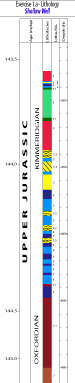 Lithofacies.
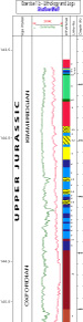 Lithofacies + Well Logs.
  Solution.
Well # 2 - Deeper region:
 Lithofacies.
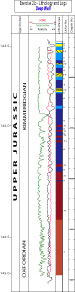 Lithofacies + Well Logs.
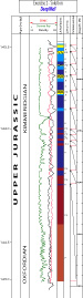 Solution.
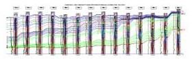
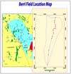 Saudi Aramco provided the above well data for this high frequency sequence stratigraphic analysis of the first two wells and the later 14 wells from an axial line of dip (NE-SW) at the crest of the Berri Field where it intersects the coast of the Arabia Gulf about 100 km north of Dhahran, Saudi Arabia. This section is approximately 55 km long and 30 km wide, with each well having gamma ray, porosity, permeability, sonic, and density log information tied to a core description and lithofacies analysis based on the original Hanifa Formation interpretation of the Berri field by the Saudi Aramco-Mobil team in 1991 and McGuire et al. (1993).
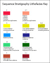 Parasequences within cored wells are defined on the basis of subdividing stratigraphic surfaces and lithology. This first exercise consists of two separate wells and a lithological key (see figure to right). Using the lithological key and well log character identify the parasequences or cycles within the well sections.
The interpretation process is divided here into 2 steps:
1. Using the well with described lithofacies, identify all parasequences (cycles). As given in the definition of cycles, each shoaling upward cycle is bounded by a maximum flooding surface. Therefore, the lower surface of the cycle is the base of the deeper lithofacies layer which overlies the top of a shallowing upward cycle. The upper boundary is the top of a shallower lithofacies layer which is overlain by a deeper lithofacies layer. Mark each cycle with a curved arrow to indicates the grain size variation and so its shoaling upward character. An arrow that moves to the left indicates that the grain size is coarser and so the water is becoming shallower.
2. Using the sonic and gamma ray logs, establish the patterns of deepening and shallowing and determine whether the cycles you identify from the cores can be tied to variations in the log character. This step is important since it enables the subsequent regional correlation to be based on specific log markers. For example, there are a few gamma ray spikes that indicate sudden deepening. You will see later that one of these spikes is identified as the most significant maximum flooding surface for the whole sequence. Overall the third order sequence character may be deduced by identifying the deepening and shoaling trend (from one mfs to the next). Additionally, some cycle boundaries also have clear log character change.
If you are confused in this exercise you should work you way through the earlier sections of:
2) parasequence correlation
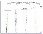
Exercise 2 - Correlate four well logs on the basis of well logs and cores used together
The objective of this exercise is to introduce the concept of well log correlation. The exercise utilizes the logs of four wells (right side is north, left side is south). The interval which is bounded by transgressive surfaces represents a complete sequence (TS to TS). All wells are datumed to the transgressive surface (TS) datum at the base of the section. The exercise is subdivided into two steps:
1. Using the well logs only:
a) For each well, identify the trends in the paleobathymetry and grain size of the lithology and the logs (shoaling or deepening) and identify parasequences (cycles) which are bounded by mfs.
b) See if you can find clear electric log events (mainly gamma log spikes) that can be identified in all or most wells. Use these markers for correlating all four wells.
c) Determine the overall profile of the section (north to south).
2. By combining the log interpretation with lithofacies cycle identification, the interpretation process can be much more definite.
a) For each well, identify all cycles.
b) For the overall lithofacies character (shallowing, deepening, thickness changes, etc.), and in combination with the interpretation of step 1, identify the third-order sequence major surfaces including the maximum flooding surface (mfs) and the sequence boundary (SB).
This exercise requires the identification of the major stratigraphic surfaces that can be correlated from well to well.
 The surfaces should be identified on the basis of the log character and the stacking patterns of the wells.
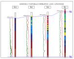 Make the correlation of the four wells on the basis of parasequences.
 Solution.
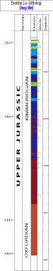
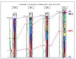
Exercise 3 - The final and complete regional sequence stratigraphic interpretation
Using the results of exercise 2, make an interpretation of all fourteen regional wells. The well spacing is approximately 4 km. The objective of this exercise is to identify the architecture of the sequence and its major systems tract components (TST, HST, SWM or LST) and to relate their occurrence to the position of the sea level. The reason for doing this is to better understand the processes that lead to the deposition of these different systems tracts.
The exercise is subdivided into two steps:
-
Interpret the well logs in order to identify the parasequences and the surfaces that subdivide them (See step 1 of exercise 2).
-
Using the character of the superimposed lithofacies, the interpretation as stated in step 2 of exercise 2. Additionally, major surfaces should be identified or confirmed by utilizing cycles geometries and their relationships to the major surfaces. For example, a maximum flooding surface may be identified as the surface on which overlying cycles downlap and aggrade then prograde. A sequence boundary (SB) may be recognized if there are terminating (truncating) cycles in the shallow regions (north), etc.
The final interpretation should provide a fairly accurate representation of the reservoir architecture and can be used for recommending hydrocarbon extraction based on juxtaposition of source, reservoir, and seal.
Unlike some of the earlier exercises this one does not use seismic but instead allows you to make an interpretation of regional sedimentary geometries from 14 (fourteen) well logs:
-
Make regional well log interpretation and identify major surfaces
-
Superimpose lithofacies and improve interpretation
-
Construct Fisher diagram based on shallow sector of the updip wells.
-
Improve and enhance lithofacies interpretation.
-
-
Produce 2D models and define best reservoir, source and seal.
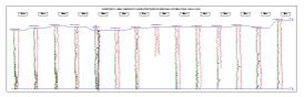 Interpretation based on well logs.
 Interpretation based on lithofacies character + well logs.
 Final Solution.
Exercise 4 - Improve correlation - the use of Fischer Diagrams
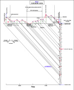
The Fischer plot is a graph with two axes. The horizontal axis represents time and the vertical axis represents thickness. Having established the length of time involved to accumulate the thickness of sediment within the section a line representing the rate of subsidence of this section is drawn across the graph from upper left to lower right, with the upper left end starting at the top of the section at the time of the initiation of deposition of the section and the lower right end terminating at the time of the termination of deposition and at the base of the section.
Then working from the base of the section up, plot the thickness of the first parasequence as a vertical line, with its base resting on the diagonal subsidence line at the time of the start of deposition of that parasequence. Now draw a further line of subsidence from the top of the vertical line representing the first parasequence to the vertical axis on the lower right. Next plot the thickness of the second parasequence as a vertical line, with its base resting on the new diagonal subsidence line at the time of the start of its deposition. Now plot another line of subsidence from the top of this parasequence to the vertical axis on the right. Repeat this process for each of the parasequences until the vertical lines for each has been plotted. When this is finished you will note that the subsidence is represented by a series of inclined parallel lines and the horizontal spacing of the vertical lines representing the parasequences is equally spaced. This is because each parasequence is assumed to have the same time duration. This oversimplification explains some of the character of this plot.
Now draw a curving line that connects the tops of the each of the vertical lines representing the thicknesses of each parasequence. This curve represents sea level position through time. Because this solution to the exercise is a smooth interpolation, this curve may it lie just below the crests of some of the parasequences. However, in this particular case it should not be inferred that the crests of these parasequences were exposed. Some exposure has been seen in the local updip stratigraphy but this is ambiguous. In the case in point the peaks or tops of the parasequences are mfs, and so might not be expected to show exposure!!! Not the spacing of the inclined subsidence lines varies. This reflects variation in the thickness of each parasequence. An increase in thickness of the parasequences means that accommodation space was increasing and may be the result of an eustatic rise or increased subsidence. If the parasequences thin then this means that there is a decrease in accommodation space and sea level is falling or subsidence is decreasing.
 Fischer Diagram cycles mapping.
 Fischer
Correlation using parasequences; parasequence set; parasequence sets; and Systems Tracts
.
The bounding surfaces that envelop and subdivide parasequences of the wells in the exercises
The Surfaces listed below can be seen in the cores and well logs of the exercise materials. You should note that there are no type 1 Sequence Boundaries in these sections
How major surfaces are identified using lithofacies character
Shelf-margin wedge (SMW) Sequence Boundary, type-2 (SB-2)
If the SMW SB-2's of the exercise data set are examined and compared to the other systems tracts they will be found to be relatively thin and so the adjacent Sequence Boundary may be ambiguous. For this reason the best means of identifying this boundary is by looking for marked changes in the trends shown by the Stacking Patterns. Goldhammer et al. (1991) noted that a SB-2 usually develops during a time at which there is a maximum decrease in the rate of development of long-term Accommodation. This occurs when is a turn around occurs from progressively thinning upward cycles to thickening upward cycles. Thus a SB-2 is to be identified on the basis of the character of Stacking Patterns including cycle thickness, facies character, lateral geometry, and early diagenetic attributes (Goldhammer et al., 1991) (Figure)
Transgressive or Drowning Surface (ts)
This surface marks the sudden deepening (increase of Relative Sea Level) and the termination or decrease in the deposition of shallow lithofacies while there is increase in the thickness of deeper water lithofacies. This surface is often marked by a hardground and or Glossifungites burrows and borings. Sometimes a reworked gravel of the shallow sediment lies on this surface.
The Maximum Flooding Surface (mfs)
The best means to identify the mfs within shallow part of the Basin (outer ramp) is to identify a definite change in stacking pattern in which the cycles change from deep facies (wackestone and packstone dominated) into shallow facies (skeletal Intraclasts). This geometrical trend can also be observed as it moves laterally shelfward.
How major Surfaces are identified using well log character
Shelf-margin wedge (SMW) Sequence Boundary, type-2 (SB-2)
An SB-2 is identified by an abrupt Gamma Ray spike (high), which corresponds to an increase in porosity either within the shelf margin or the Basin region
Transgressive or Drowning Surface (ts)
The Drowning Surface can also be identified by an abrupt Gamma Ray Log spike (high) marking deepening (significant change in Lithology); an increase of sonic velocity; and sudden decrease in porosity to very low values (5% or less) throughout the section. All these properties are indicators of a sudden deepening in the depositional setting (increase of Relative Sea Level).
The Maximum Flooding Surface (mfs)
An mfs is identified in the section by an abrupt gamma ray spike of logs from wells within the basin. It should be noted that an mfs becomes increasingly difficult to identify within sediments were deposited close to and within the shelf setting since in these localities only contain shallow shelf carbonate facies and no radioactive shales are present. Despite this lack of shale a gamma ray spike can still be recognized, particularly where this has been amplified to aid in its identification.
Fischer Diagrams
Fischer plots can be used successfully to extract the 3rd-order and higher sea level fluctuations from high frequency cycles identified on the section. These plots illustrate long-term accommodation changes similar to those explained by Goldhammer et al. (1991) and "reveal systematic changes in accommodation by plotting successive deviations in cycle thickness from the average cycle thickness" (Read and Goldhammer, 1988). Fischer diagrams (plots) can be constructed to build third order sea level curves that can then be comparing to the Haq et al (1987) sea curve. Another important use for these plots is to establish the role of subsidence within the depositional setting. This is achieved by comparing plots for different localities within a basin. The wells selected for the exercise penetrate the shallowest portion of the section. Selecting wells to make Fischer plots from the deep water parts of the basin does not work out so well. This is because though the lime mudstone parasequences that form the basin fill have a cyclic character it is difficult to establish their relationship to water depth or time, key components to the Fischer plot.
The Fischer plots should be constructed based on the assumption that each cycle (parasequence) was deposited over times of equal duration and their subsidence rate were linear (sedimentation = subsidence). Any deviation from the horizontal datum reflected either eustatic sea level change or changes in subsidence rate (Read and Goldhammer, 1988). Since the duration in which these carbonate were deposited was relatively short, it is logical to infer that the primary controlling factor that lead to these deposits was short-term eustatic sea level fluctuation. The average cycle period (time/number of cycles) can also be determined if an exact duration is determined for any part of the section. For shallow water carbonates that experience exposure the cycle thickness can be used to infer a rise in the Relative Sea Level and an increase in the resultant Accommodation space.
The sea level curve rise-fall that can be determined from the Fisher Plots can be used to illustrate the relationship between sea-level changes and cycle thickness in response to the creation of accommodation space. The two diagrams provided with the exercises clearly show that during a sea-level rise, the cycle thickens; on the other hand, when sea level falls, the cycle thins.
Fourth-order sequences can be identified from the constructing the Fischer diagrams. Each of these sequences is bounded by a type-2 sequence boundary and is recognized on the diagram at the maximum sea level fall inflection point. Each of the 4th order sequences has a recognizable maximum flooding surface.